Explore market data.
[1]:
from mypo import Loader, SamplingMethod
[2]:
loader = Loader()
loader.get('VOO', expense_ratio=0.0003)
loader.get('EDV', expense_ratio=0.0007)
[3]:
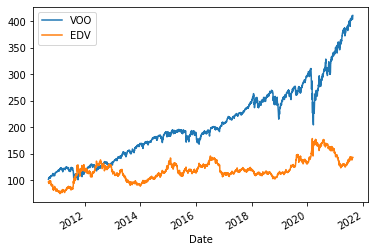
market = loader.get_market()
market.get_raw().plot()
[3]:
<AxesSubplot:xlabel='Date'>
[4]:
print(market.get_first_date())
print(market.get_last_date())
2010-09-09 00:00:00
2021-08-23 00:00:00
[5]:
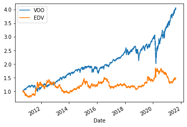
market.get_normalized_prices().plot()
[5]:
<AxesSubplot:xlabel='Date'>
[6]:
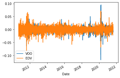
rate_of_change = market.get_rate_of_change()
rate_of_change.plot()
[6]:
<AxesSubplot:xlabel='Date'>
[7]:
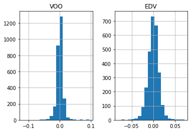
rate_of_change.hist(bins=20)
[7]:
array([[<AxesSubplot:title={'center':'VOO'}>,
        <AxesSubplot:title={'center':'EDV'}>]], dtype=object)
[8]:
rate_of_change.describe()
[8]:
| VOO | EDV | |
|---|---|---|
| count | 2757.000000 | 2757.000000 |
| mean | 0.000566 | 0.000228 |
| std | 0.010724 | 0.012988 |
| min | -0.117388 | -0.081443 |
| 25% | -0.003364 | -0.007066 |
| 50% | 0.000740 | 0.000611 |
| 75% | 0.005509 | 0.007834 |
| max | 0.095364 | 0.071497 |
[9]:
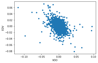
rate_of_change.plot.scatter(
    x = rate_of_change.columns[0],
    y = rate_of_change.columns[1]
)
[9]:
<AxesSubplot:xlabel='VOO', ylabel='EDV'>
[10]:
rate_of_change.corr()
[10]:
| VOO | EDV | |
|---|---|---|
| VOO | 1.000000 | -0.419186 |
| EDV | -0.419186 | 1.000000 |
[11]:
years = market.resample(SamplingMethod.YEAR)
years.get_rate_of_change()
[11]:
| VOO | EDV | |
|---|---|---|
| Date | ||
| 2013-12-31 | 0.297361 | -0.234741 |
| 2014-12-31 | 0.113804 | 0.396192 |
| 2015-12-31 | -0.007803 | -0.086655 |
| 2016-12-31 | 0.098326 | -0.033392 |
| 2017-12-31 | 0.194730 | 0.105739 |
| 2018-12-31 | -0.063109 | -0.062237 |
| 2019-12-31 | 0.287150 | 0.145602 |
| 2020-12-31 | 0.161900 | 0.171719 |